How To Make A Cashier Count Chart In Excel / Making Change By Counting Up Worksheets Teaching Resources Tpt. Control charts are statistical visual measures to monitor how your process is running over a given period of time. If you need to create or update a gantt chart for recurring communications, it will be simpler and faster than any other chart used. The only difference is in formatting. You can easily make a pie chart in excel to make data easier to understand. Making statements based on opinion;
If you need to create or update a gantt chart for recurring communications, it will be simpler and faster than any other chart used. As you'll see, creating charts is very easy. How to create a chart by count of values in excel : In excel 2007, 2010 or 2013, you can create a table to expand the data range, and the chart will update automatically. If you don't have excel 2016 or later, simply create a pareto chart by combining a column chart and a line graph.
How To Create A Chart By Count Of Values In Excel from lookaside.fbsbx.com Click the insert tab, click bar chart, and then click clustered bar (in 2016 versions, hover your cursor over the options to display a sample of how the chart will appear). Using a graph is a great way to present your data in an effective, visual way. How to create a column chart. In excel 2007, 2010 or 2013, you can create a table to expand the data range, and the chart will update automatically. Task suppose you are asked to show both frequency and percentage distribution in the same bar or column chart. How to create a chart by count of values in excel : On the insert tab, in the charts group, click the line symbol. First, select a number in column b.
I am using ms office 2010.
A simple chart in excel can say more than a sheet full of numbers. In the create table dialog box, if your data has headers, please check my table has headers option, then click ok. In this video tutorial, you'll see how to create a simple pie graph in excel. Map charts have gotten even easier with geography data types.simply input a list of geographic values, such as country, state, county, city, postal code, and so on, then select your list and go to the data tab > data types > geography.excel will automatically convert your data to a geography data type, and will include properties relevant to that data that. If you don't have excel 2016 or later, simply create a pareto chart by combining a column chart and a line graph. First, select a number in column b. To plot specific data into a chart, you can also select the data. I am using ms office 2010. Excel has a variety of graphs and charts that can be used to represent data in different ways. If the specific day of the month is inconsequential, such as the billing date for monthly bills. I only know use excel a little bit. Let's understand the working of it with the below simple steps. Formulas are the key to getting things done in excel.
You can easily make a pie chart in excel to make data easier to understand. Home » advanced excel » excel charts » count and percentage in a column chart. It also enables users to then click ok. For a refresher on making standard graphs and charts in excel, check out this helpful article: The simplest is to do a pivotchart.
Cashbook In Excel Youtube from i.ytimg.com For the first formula, i need to count all responses. I am using ms office 2010. Don't worry, as it is easy to do. On the insert tab, in the charts group, click the line symbol. Select the data and insert a column chart or bar chart. Formulas are the key to getting things done in excel. Click the insert tab, click bar chart, and then click clustered bar (in 2016 versions, hover your cursor over the options to display a sample of how the chart will appear). This tutorial will show you how to create stock charts in excel 2003.
Let's understand the gantt chart and how to create it.
How to make a cashier count chart in excel : You can create a chart for your data in excel for the web. If the specific day of the month is inconsequential, such as the billing date for monthly bills. Select the entire data set, including the supporting columns. In this example it is a net worth and its change over last years. It also enables users to then click ok. To highlight the highest value in a bar or column chart we use almost the same technique as the excel line chart. Value and percentage in same column chart: Control charts are statistical visual measures to monitor how your process is running over a given period of time. How to create a bar chart. How to make a cashier count chart in excel : To create a line chart, execute the following steps. As you can see in the screenshot below, start date is already added under legend entries (series).and you need to add duration there as well.
Next, sort your data in descending order. Let's understand the working of it with the below simple steps. It also enables users to then click ok. Add the autofilter icon to the quick access toolbar. For the first formula, i need to count all responses.
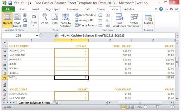
Free Cashier Balance Sheet Template For Excel 2013 from cdn.free-power-point-templates.com In this example it is a net worth and its change over last years. Add the autofilter icon to the quick access toolbar. If you don't have excel 2016 or later, simply create a pareto chart by combining a column chart and a line graph. Ms excel has a bar chart feature that can be used to make an excel gantt chart. The map chart in excel works best with large areas like counties, states, regions, countries, and continents. To plot specific data into a chart, you can also select the data. The argument you are entering at the moment is highlighted in bold. Formulas are the key to getting things done in excel.
This step is not required, but it will make the formulas easier to write.
Select the data range and click table under insert tab, see screenshot: Add the autofilter icon to the quick access toolbar. As you can see in the screenshot below, start date is already added under legend entries (series).and you need to add duration there as well. The only difference is in formatting. Using a graph is a great way to present your data in an effective, visual way. The process only takes 5 steps. I only know use excel a little bit. Count values with conditions using this amazing function. In this video tutorial, you'll see how to create a simple pie graph in excel. The select data source window will open. You can use the countifs function in excel to count cells in a single range with a single condition as well as in multiple ranges with multiple conditions. Microsoft excel offers the autofill feature to enable you to insert a sequence of numbers and avoid the tedious task of manually entering a value in every cell. You can easily make a pie chart in excel to make data easier to understand.
Share :
Post a Comment
for "How To Make A Cashier Count Chart In Excel / Making Change By Counting Up Worksheets Teaching Resources Tpt"


Post a Comment for "How To Make A Cashier Count Chart In Excel / Making Change By Counting Up Worksheets Teaching Resources Tpt"